Choosing the Right Loss Function for your ML Problem

Choosing the right loss function is one of those decisions that can make or break your model. Get it wrong, and your network might struggle to learn anything useful. Get it right, and training becomes smooth and efficient.

The good news? Once you understand a few key principles, the choice becomes straightforward. The loss function you need depends on what you’re predicting and how your targets are formatted — not on whether you’re using a CNN, MLP, or Transformer.

This guide covers loss functions across the modern deep learning landscape: classification, regression, LLMs, object detection, segmentation, generative models, and more. The detailed examples focus on classification (the most common case), but the quick reference covers everything you’ll encounter in practice.

---

Quick Decision Guide

Before diving into the details, here’s the comprehensive cheat sheet organized by task type:

Classification

Scenario	Loss Function
Single-label, multi-class (image classification, sentiment)	nn.CrossEntropyLoss
Binary (yes/no, spam detection)	nn.BCEWithLogitsLoss
Multi-label (tagging, multi-object)	nn.BCEWithLogitsLoss
Token classification (NER, POS tagging)	nn.CrossEntropyLoss + ignore_index
Class imbalance	Add weight= or pos_weight=
Extreme imbalance (object detection)	Focal Loss
Want softer predictions	Add label_smoothing
Margin-based (SVM-style)	nn.MultiMarginLoss

Regression

Scenario	Loss Function
Standard regression	nn.MSELoss (L2)
Robust to outliers	nn.L1Loss (MAE) or nn.SmoothL1Loss (Huber)
Bounding box regression (object detection)	nn.SmoothL1Loss or IoU Loss
Time series forecasting	nn.MSELoss, nn.L1Loss, or Quantile Loss

Language Models (LLMs / Transformers)

Scenario	Loss Function
Next-token prediction (GPT-style)	nn.CrossEntropyLoss on vocabulary
Masked language modeling (BERT-style)	nn.CrossEntropyLoss on masked tokens
Sequence-to-sequence (translation, summarization)	nn.CrossEntropyLoss + ignore_index for padding
RLHF / preference learning	Reward model + PPO policy loss
Contrastive learning (CLIP, sentence embeddings)	Contrastive Loss / InfoNCE

Computer Vision — Detection & Segmentation

Scenario	Loss Function
Object detection (YOLO, SSD)	Classification CE + Localization (Smooth L1 / IoU)
Semantic segmentation	nn.CrossEntropyLoss (per-pixel) or Dice Loss
Instance segmentation	CE + Mask Loss + Box Loss
Imbalanced segmentation	Dice Loss, Focal Loss, or Tversky Loss

Generative Models

Scenario	Loss Function
Autoencoders (VAE)	Reconstruction (MSE/BCE) + KL Divergence
GANs	Adversarial Loss (Generator + Discriminator)
Diffusion models (Stable Diffusion)	Noise prediction loss (MSE on predicted noise)
Image-to-image (Pix2Pix, CycleGAN)	L1/L2 + Adversarial + Perceptual Loss
Style transfer	Content Loss + Style Loss (Gram matrices)

Embeddings & Similarity

Scenario	Loss Function
Metric learning (face recognition)	Triplet Loss, Contrastive Loss
Sentence embeddings	Multiple Negatives Ranking Loss, Cosine Similarity Loss
Siamese networks	Contrastive Loss

Now let’s see the most common ones in action with PyTorch code.

---

Single-Label, Multi-Class Classification

This is the most common scenario: your model outputs one class from a set of possibilities. Think image classification (“is this a cat, dog, or bird?”) or sentiment analysis (“positive, negative, or neutral”).

The go-to loss here is Cross-Entropy Loss. Mathematically, for a single sample:

\[\mathcal{L}_{CE} = -\log p(y) \quad \text{where} \quad p = \text{softmax}(z)\]

The key insight: PyTorch’s CrossEntropyLoss expects raw logits — it handles the softmax internally. Don’t apply softmax yourself, or you’ll get wrong gradients.

CNN Example (Images)

import torch
import torch.nn as nn

class TinyCNN(nn.Module):
    def __init__(self, num_classes=10):
        super().__init__()
        self.net = nn.Sequential(
            nn.Conv2d(3, 32, 3, padding=1),  # [B, 32, H, W]
            nn.ReLU(),
            nn.MaxPool2d(2),                 # downsample
            nn.Conv2d(32, 64, 3, padding=1),
            nn.ReLU(),
            nn.AdaptiveAvgPool2d(1),         # [B, 64, 1, 1]
            nn.Flatten(),                    # [B, 64]
            nn.Linear(64, num_classes)       # logits
        )

    def forward(self, x):
        return self.net(x)

model = TinyCNN(num_classes=10)

# Fake batch
x = torch.randn(8, 3, 64, 64)
y = torch.randint(0, 10, (8,))  # class indices

criterion = nn.CrossEntropyLoss()  # logits + class indices
logits = model(x)
loss = criterion(logits, y)
loss.backward()

MLP Example (Tabular Data)

import torch
import torch.nn as nn

class TinyMLP(nn.Module):
    def __init__(self, in_features=20, num_classes=4):
        super().__init__()
        self.net = nn.Sequential(
            nn.Linear(in_features, 64),
            nn.ReLU(),
            nn.Linear(64, 32),
            nn.ReLU(),
            nn.Linear(32, num_classes)  # logits
        )

    def forward(self, x):
        return self.net(x)

model = TinyMLP(in_features=20, num_classes=4)

x = torch.randn(16, 20)
y = torch.randint(0, 4, (16,))

loss = nn.CrossEntropyLoss()(model(x), y)
loss.backward()

Same task, same loss — the architecture doesn’t change the objective.

Transformer Example (Sequence Classification)

Here’s a minimal encoder-style classifier:

import torch
import torch.nn as nn

class TinyTransformerClassifier(nn.Module):
    def __init__(self, vocab_size=1000, d_model=64, nhead=4, num_layers=2, num_classes=3):
        super().__init__()
        self.embedding = nn.Embedding(vocab_size, d_model)

        encoder_layer = nn.TransformerEncoderLayer(
            d_model=d_model,
            nhead=nhead,
            batch_first=True
        )
        self.encoder = nn.TransformerEncoder(encoder_layer, num_layers=num_layers)

        self.classifier = nn.Linear(d_model, num_classes)

    def forward(self, input_ids):
        # input_ids: [B, T]
        x = self.embedding(input_ids)       # [B, T, d_model]
        x = self.encoder(x)                 # [B, T, d_model]
        pooled = x[:, 0]                    # simple CLS-like pooling
        return self.classifier(pooled)      # logits

model = TinyTransformerClassifier()

input_ids = torch.randint(0, 1000, (8, 32))
labels = torch.randint(0, 3, (8,))

criterion = nn.CrossEntropyLoss()
logits = model(input_ids)
loss = criterion(logits, labels)
loss.backward()

Transformer, CNN, MLP — the loss function stays the same because the task is the same.

---

Binary Classification

When you have exactly two classes, you could use CrossEntropyLoss with two output neurons. But the cleaner approach is a single output neuron with BCEWithLogitsLoss:

\[\mathcal{L}_{BCE} = -\big(y\log\sigma(z) + (1-y)\log(1-\sigma(z))\big)\]

The “WithLogits” part means it applies sigmoid internally — so again, don’t apply sigmoid yourself.

Binary CNN Example

import torch
import torch.nn as nn

class BinaryCNN(nn.Module):
    def __init__(self):
        super().__init__()
        self.features = nn.Sequential(
            nn.Conv2d(3, 16, 3, padding=1),
            nn.ReLU(),
            nn.AdaptiveAvgPool2d(1),
            nn.Flatten(),
        )
        self.head = nn.Linear(16, 1)  # single logit

    def forward(self, x):
        return self.head(self.features(x)).squeeze(-1)  # [B]

model = BinaryCNN()
x = torch.randn(8, 3, 64, 64)
y = torch.randint(0, 2, (8,)).float()

criterion = nn.BCEWithLogitsLoss()
logits = model(x)
loss = criterion(logits, y)
loss.backward()

---

Multi-Label Classification

Sometimes each sample can have multiple labels simultaneously. Think tagging a movie as both “action” and “comedy”, or detecting multiple objects in an image.

The solution: treat each label as an independent binary classification. Use BCEWithLogitsLoss with targets shaped [batch, num_labels]:

import torch
import torch.nn as nn

B, L = 4, 5
logits = torch.randn(B, L)  # raw scores for each label
targets = torch.randint(0, 2, (B, L)).float()

criterion = nn.BCEWithLogitsLoss()
loss = criterion(logits, targets)
loss.backward()

Handling Imbalanced Labels

If some labels are rare, use pos_weight to give them more importance:

pos_weight = torch.tensor([3.0, 1.0, 2.0, 5.0, 1.0])  # example weights
criterion = nn.BCEWithLogitsLoss(pos_weight=pos_weight)
loss = criterion(logits, targets)

---

Token Classification (NER, POS Tagging)

For tasks like Named Entity Recognition, you’re doing single-label classification per token. The twist: you need to ignore padding tokens. That’s what ignore_index is for:

import torch
import torch.nn as nn

B, T, C = 2, 6, 4
logits = torch.randn(B, T, C)  # [batch, tokens, classes]
targets = torch.randint(0, C, (B, T))

PAD_LABEL = -100
targets[0, -2:] = PAD_LABEL  # pretend last two tokens are padding

criterion = nn.CrossEntropyLoss(ignore_index=PAD_LABEL)
loss = criterion(logits.view(-1, C), targets.view(-1))
loss.backward()

The loss is computed only on real tokens, not padding.

---

Dealing with Class Imbalance

Real-world datasets are rarely balanced. Here are three tools, in order of escalation:

1. Weighted Cross-Entropy

Give more weight to underrepresented classes:

import torch
import torch.nn as nn

class_weights = torch.tensor([1.0, 2.0, 5.0])  # rare class gets 5x weight
criterion = nn.CrossEntropyLoss(weight=class_weights)

2. pos_weight for Binary/Multi-Label

pos_weight = torch.tensor([4.0])  # positive samples count 4x
criterion = nn.BCEWithLogitsLoss(pos_weight=pos_weight)

3. Focal Loss (For Extreme Imbalance)

When you have severe imbalance (like 1:1000 ratios in object detection), Focal Loss down-weights easy examples so the model focuses on hard ones:

\[FL(p_t) = -(1-p_t)^\gamma \log(p_t)\]

The γ parameter (typically 2.0) controls how much to focus on hard examples. Torchvision provides this out of the box:

import torch
from torchvision.ops import sigmoid_focal_loss

logits = torch.randn(8)               # binary logits
targets = torch.randint(0, 2, (8,)).float()

# alpha balances pos/neg, gamma focuses on hard examples
loss = sigmoid_focal_loss(
    inputs=logits,
    targets=targets,
    alpha=0.25,
    gamma=2.0,
    reduction="mean"
)
loss.backward()

---

Label Smoothing

Hard labels (0 or 1) can make models overconfident. Label smoothing softens the targets slightly, which often improves generalization:

import torch
import torch.nn as nn

criterion = nn.CrossEntropyLoss(label_smoothing=0.1)

With label_smoothing=0.1, the target becomes 90% on the correct class and 10% spread across others. This acts as a regularizer.

---

Margin-Based Loss

If you prefer SVM-style hinge loss for multi-class problems, MultiMarginLoss is available:

import torch
import torch.nn as nn

logits = torch.tensor([[0.1, 0.2, 0.4, 0.8]])  # [B, C]
targets = torch.tensor([3])

criterion = nn.MultiMarginLoss(margin=1.0, p=1)
loss = criterion(logits, targets)
loss.backward()

This penalizes predictions that don’t have a sufficient margin from competing classes.

---

Common Gotchas

A few mistakes I see repeatedly:

Don’t double-apply activations. CrossEntropyLoss expects logits — if you apply softmax first, you’ll get wrong gradients. Same with BCEWithLogitsLoss and sigmoid.

Match your target types. CrossEntropyLoss wants class indices as LongTensor. BCEWithLogitsLoss wants floats in [0, 1].

Check your shapes. For CE: logits are [batch, classes], targets are [batch]. For BCE: both are [batch, labels].

---

Wrapping Up

Loss function selection doesn’t have to be mysterious. For classification:

• One class per sample → CrossEntropyLoss
• Binary yes/no → BCEWithLogitsLoss
• Multiple labels per sample → BCEWithLogitsLoss
• Imbalanced data → Add weights or use Focal Loss
• Want regularization → Try label smoothing

The architecture (CNN, Transformer, MLP) doesn’t change the loss — the task does. Once you internalize this, picking the right loss becomes second nature.

---

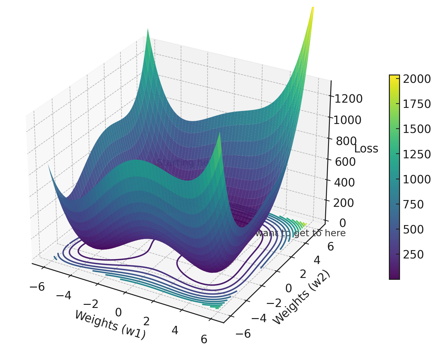
Bonus: Visualizing the Loss Landscape

The hero image for this post was generated with the following script, which renders a 3D loss surface using the Himmelblau function — a classic non-convex landscape that resembles real neural network loss surfaces:

import torch
import matplotlib.pyplot as plt
from mpl_toolkits.mplot3d import Axes3D  # noqa: F401

# Toy non-convex loss surface: Himmelblau function
# Looks similar to classic "NN loss landscape" illustrations.
def himmelblau(w1, w2):
    return (w1**2 + w2 - 11)**2 + (w1 + w2**2 - 7)**2

# Create a grid over two "weights"
w1 = torch.linspace(-6, 6, 200)
w2 = torch.linspace(-6, 6, 200)
W1, W2 = torch.meshgrid(w1, w2, indexing="ij")
L = himmelblau(W1, W2)

# Convert to numpy for plotting
W1n = W1.numpy()
W2n = W2.numpy()
Ln = L.numpy()

# Mark a start point and a target minimum
start = torch.tensor([-4.5, 4.5])
target = torch.tensor([3.0, 2.0])  # known minimum vicinity

start_loss = himmelblau(start[0], start[1]).item()
target_loss = himmelblau(target[0], target[1]).item()

# Plot the surface
fig = plt.figure(figsize=(10, 6.5))
ax = fig.add_subplot(111, projection="3d")

surf = ax.plot_surface(
    W1n, W2n, Ln,
    linewidth=0,
    antialiased=True,
    cmap="viridis",
    alpha=0.95
)

# Add floor contours for readability
z_offset = Ln.min() - 10
ax.contour(W1n, W2n, Ln, zdir="z", offset=z_offset, levels=15)

# Scatter markers for start/goal
ax.scatter(start[0].item(), start[1].item(), start_loss, s=60, marker="o")
ax.scatter(target[0].item(), target[1].item(), target_loss, s=80, marker="o")

# Text annotations
ax.text(start[0].item(), start[1].item(), start_loss + 15, "Starting here")
ax.text(target[0].item(), target[1].item(), target_loss + 15, "We want to get to here")

# Labels similar to classic "loss landscape" figures
ax.set_xlabel("Weights (w1)")
ax.set_ylabel("Weights (w2)")
ax.set_zlabel("Loss")

# Ensure the contour floor is visible
ax.set_zlim(z_offset, Ln.max() * 0.6)

# View angle
ax.view_init(elev=28, azim=-60)

# Colorbar
fig.colorbar(surf, shrink=0.6, pad=0.08)

# Save locally
plt.savefig("loss_landscape_3d.png", dpi=220, bbox_inches="tight")
plt.close()

print("Saved: loss_landscape_3d.png")

This visualization shows the challenge of optimization: navigating a complex, non-convex surface with multiple local minima to find the global minimum. The loss function defines what this surface looks like — the optimizer determines how we traverse it.

---

References

• PyTorch CrossEntropyLoss
• PyTorch BCEWithLogitsLoss
• PyTorch MultiMarginLoss
• Torchvision Focal Loss
• Sambasivarao K’s original overview