Mastering Language Modeling: From N-grams to RNNs and Beyond

A modern language model must handle vast contexts, share parameters efficiently, and overcome the vanishing-gradient issues that plagued early RNNs. Count-based n-grams hit a combinatorial wall: storage blows up and sparsity kills generalization (Limitations of N-gram Language Models and the Need for Neural Networks). Bengio et al.’s fixed-window neural LM introduced embeddings and a Softmax over concatenated vectors, yet still used separate weights per position (A Neural Probabilistic Language Model). Elman RNNs unify this by reusing input, recurrent, and output matrices $U,W,V$ at every time step, making the model compact and context-flexible (Simple Recurrent Networks). However, simple RNNs suffer vanishing gradients, effectively “forgetting” information more than ~7 steps back (Why do RNNs have Short-term Memory?). LSTMs fix this with additive cell-state updates gated by forget, input, and output gates, preserving long-term dependencies (LSTM and its equations). Training minimizes average cross-entropy—whose exponentiation yields perplexity (lower is better) (en.wikipedia.org, medium.com)—via Backpropagation Through Time, often truncated for efficiency (neptune.ai). RNNs also power speech, translation, and time-series tasks, and at scale demand tricks like Facebook’s adaptive softmax for billion-word vocabularies (engineering.fb.com). Despite remedies like gradient clipping for exploding gradients (arxiv.org), vanilla RNNs remain eclipsed by LSTM/GRU and now Transformers (en.wikipedia.org).

---

Why Go Beyond N-grams?

N-gram models estimate $P(w_t\mid w_{t-n+1}^{t-1})$ using counts, but as $n$ grows the number of possible sequences explodes exponentially, leading to severe sparsity and massive storage requirements (medium.com). Smoothing helps (e.g., Kneser-Ney), yet cannot capture dependencies beyond its fixed window, limiting context to a handful of words (linkedin.com). Moreover, count-based methods assign zero probability to unseen n-grams, forcing back-off strategies that degrade fluency and accuracy (jmlr.org).

Fixed-Window Neural Language Models

Bengio et al. (2003) introduced a neural LM that embeds the previous $n$ words into continuous vectors, concatenates them, and passes through a hidden layer $h = \tanh(W^\top [e_{t-n+1};\dots;e_{t-1}] + b)$ followed by

\[P(w_t \mid w_{t-n+1}^{t-1}) = \frac{\exp(v_{w_t}^\top h + c_{w_t})}{\sum_{w'} \exp(v_{w'}^\top h + c_{w'})},\]

showing better generalization than n-grams by smoothing via embeddings instead of counts (jmlr.org). Yet this model still fixes the context length and uses separate parameters for each position in the window, limiting scalability.

Elman RNNs: Shared Weights & Variable Context

Architecture & Math

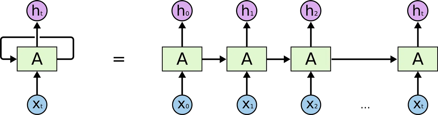
Elman RNNs process one token at a time, updating a hidden state $h_t$ that in theory encodes all history:

\[\begin{aligned} h_t &= \tanh(Ux_t + Wh_{t-1} + b_h),\\ y_t &= Vh_t + b_y,\\ P(w_{t+1}\!\mid\!w_{1:t}) &= \mathrm{Softmax}(y_t). \end{aligned}\]

Here, $U\in\mathbb{R}^{d_h\times d_x}$, $W\in\mathbb{R}^{d_h\times d_h}$, and $V\in\mathbb{R}^{|\mathcal V|\times d_h}$ are reused at every time step, sharing parameters across positions and allowing arbitrary-length context without blowing up model size (web.stanford.edu).

graph TD
    %% Nodes with KaTeX
    Xt[$$X_t$$]
    Ht[$$h_t$$]
    Yt[$$Y_t$$]

    %% Edges
    Xt --> Ht
    Ht --> Yt
    Ht -.-> Ht

    %% Styling
    style Xt fill:#1f78b4,stroke:#000,stroke-width:2px
    style Ht fill:#33a02c,stroke:#000,stroke-width:2px
    style Yt fill:#e31a1c,stroke:#000,stroke-width:2px

Above the representation of a Simple Recurrent Nets (Elman nets). The hidden layer has a recurrence as part of its input. The activation value $h_t$ depends on $x_t$ but also $h_{t-1}$!

Short-Term Memory & “Forgetting”

Despite its theoretical power, training via Backpropagation Through Time multiplies gradients by the recurrent Jacobian $\partial h_t/\partial h_{t-1}$ many times. When the largest singular value of $W$ is <1, gradients shrink exponentially, effectively wiping out signals from >7 steps back in practice (medium.com). This vanishing-gradient issue means simple RNNs primarily “remember” their most recent hidden state, forgetting earlier inputs (reddit.com).

Long Short-Term Memory (LSTM)

LSTMs introduce a cell state $c_t$ and three gates—forget $f_t$, input $i_t$, and output $o_t$—that control how information is added or removed:

\[\begin{aligned} f_t &= \sigma(W_f x_t + U_f h_{t-1} + b_f),\\ i_t &= \sigma(W_i x_t + U_i h_{t-1} + b_i),\\ o_t &= \sigma(W_o x_t + U_o h_{t-1} + b_o),\\ \tilde c_t &= \tanh(W_c x_t + U_c h_{t-1} + b_c),\\ c_t &= f_t \odot c_{t-1} + i_t \odot \tilde c_t,\\ h_t &= o_t \odot \tanh(c_t). \end{aligned}\]

The additive update to $c_t$ preserves gradient flow over long sequences, effectively solving the vanishing-gradient problem and giving LSTMs true long-term memory (medium.com).

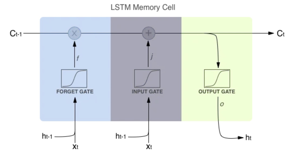LSTM memory cell source medium.com

Training Objective: Cross-Entropy & Perplexity

We train by minimizing average cross-entropy over a dataset of $N$ words ${w_i}$:

\[\mathcal{L} = -\frac{1}{N}\sum_{i=1}^N \log q(w_i),\]

where $q(w_i)$ is the model’s predicted probability (en.wikipedia.org, medium.com). Exponentiating this gives perplexity:

\[\mathrm{Perplexity} = \exp(\mathcal{L}),\]

which measures model uncertainty—lower is better (medium.com).

Backpropagation Through Time (BPTT) & Truncation

Training involves unrolling the RNN for $T$ steps and applying standard backprop on the expanded graph, summing gradients for shared weights $U,W$ across all steps. To reduce memory and computation, one uses truncated BPTT, backpropagating through only the last $k\ll T$ steps without severely harming performance (medium.com).

Other Uses of RNNs

Beyond language modeling, RNNs excel at any sequential signal:

• Speech recognition & synthesis, modeling audio frames over time
• Time-series forecasting, leveraging hidden states to predict stock prices or sensor data
• Machine translation, via encoder–decoder RNNs that map source to target sequences (jmlr.org)

RNNs in Machine Translation

Encoder–decoder RNNs encode a source sentence into a vector, then decode it into a target sentence, forming the basis of early neural MT systems and paving the way for end-to-end translation pipelines (jmlr.org).

Scaling to Billions of Words: Adaptive Softmax

Training on billion-word corpora with million-word vocabularies is intensive. Facebook AI Research’s adaptive softmax clusters rare words to reduce per-step computation on GPUs, achieving efficiency close to full Softmax while slashing training time (engineering.fb.com, arxiv.org).

Limitations: Exploding Gradients & Clipping

In addition to vanishing gradients, RNNs can suffer exploding gradients, where errors grow unbounded during BPTT. The standard remedy is gradient clipping—rescaling gradients when their norm exceeds a threshold—to stabilize training (arxiv.org).

Conclusion & Next Steps

RNN LMs marked a breakthrough beyond n-grams by sharing parameters across time and handling arbitrary contexts, but vanilla RNNs remain handicapped by short-term memory. Gated architectures like LSTM/GRU overcame this, and efficient approximations (adaptive softmax) enabled scaling. In the next post, we’ll dive deeper into LSTM/GRU variants and unveil the Transformer revolution, which now dominates sequence modeling (en.wikipedia.org).

---