What Is a Tensor? A Practical Guide for AI Engineers

When dealing with deep learning, we quickly encounter the word tensor. But what exactly is a tensor? Is it just a fancy name for an array? A mathematical object from physics? Both?

This guide takes you on a journey from intuitive understanding to practical implementation. We’ll explore tensors through four lenses:

1. The intuitive view: Understanding vectors and tensors through Dan Fleisch’s brilliant explanation
2. The computational view: How NumPy handles multi-dimensional arrays

3. The ML practitioner’s view: Working with tensors in PyTorch

Building Intuition — Vectors and Tensors Explained

“What’s a tensor?” — The question Dan Fleisch set out to answer in his book - A Student’s Guide to Vectors and Tensors

The best route to understanding tensors starts with understanding vectors. Not just as “arrays of numbers,” but as geometric objects with components and basis vectors.

Understanding Vectors Through Components

Think of a 3D Cartesian coordinate system with x, y, and z axes. This coordinate system comes with basis vectors (unit vectors):

• x̂ (or eₓ): unit vector in the x direction
• ŷ (or eᵧ): unit vector in the y direction
• ẑ (or eᵤ): unit vector in the z direction

Each basis vector has length 1 and points along its axis.

Any vector A in 3D space can be written as:

A = Aₓ x̂ + Aᵧ ŷ + Aᵤ ẑ

Where:

• (Aₓ, Aᵧ, Aᵤ) are the components — the numbers
• (x̂, ŷ, ẑ) are the basis vectors — the directions

Visualizing Vector Components

Dan Fleisch uses a beautiful analogy: imagine shining a light perpendicular to an axis. The shadow the vector casts on that axis is its component along that direction.

To find the x-component: shine light parallel to the y-axis (perpendicular to x). The shadow on the x-axis is Aₓ.

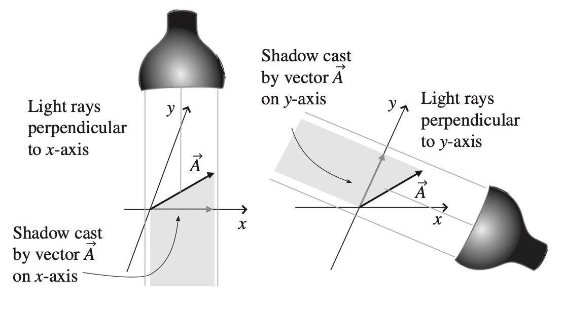Projections using light sources perpendicular to x- and y-axes - image source A Student’s Guide to Vectors and Tensors

Alternatively, think of it as: “How many x̂ unit vectors and how many ŷ unit vectors would it take to get from the base to the tip of this vector?”

This is profound because it reveals:

A vector is a geometric object.
Components depend on your coordinate system; the vector itself does not.

If you rotate your coordinate system, both the basis vectors and the components change — but the actual arrow in space remains the same.

From Vectors to Tensors: The Rank System

Now we can understand the classification:

• Scalar (rank-0 tensor): No directional information, no index needed
  • Example: temperature = 42
• Vector (rank-1 tensor): One directional indicator, one index
  • Components: Aᵢ where i ∈ {x, y, z}
  • Example: velocity = [3, 4, 0]
• Rank-2 tensor: Two directional indicators, two indices
  • Components: Tᵢⱼ where i, j ∈ {x, y, z}
  • In 3D: 3 × 3 = 9 components
  • Example: stress tensor, Jacobian matrix
• Rank-3 tensor: Three directional indicators, three indices
  • Components: Tᵢⱼₖ where i, j, k ∈ {x, y, z}
  • In 3D: 3 × 3 × 3 = 27 components

Tensor classification - image source Avnish’s Blog

Why Do We Need Higher-Rank Tensors?

Consider stress inside a solid object. You might have surfaces with area vectors pointing in the x, y, or z direction. On each surface, forces can act in the x, y, or z direction.

To fully characterize all possible forces on all possible surfaces, you need 9 components with two indices:

• Tₓₓ: x-directed force on a surface whose normal points in x
• Tᵧₓ: x-directed force on a surface whose normal points in y
• And so on…

This is a rank-2 tensor — the stress tensor.

The Power of Tensors: Coordinate Independence

Here’s what makes tensors “the facts of the universe” (as mathematician Lillian Lieber called them):

All observers, in all reference frames, agree on the combination of components and basis vectors.

They may disagree on the individual components, and on what the basis vectors are, but the components transform in just such a way to keep the combined result (the actual tensor) the same for everyone.

This is why tensors appear everywhere in physics: they express physical laws in a coordinate-free way that all observers agree on.

---

Tensors in NumPy — From Theory to Arrays

Now let’s bring this down to code. In practice, when we work with tensors in machine learning, we’re working with multi-dimensional arrays.

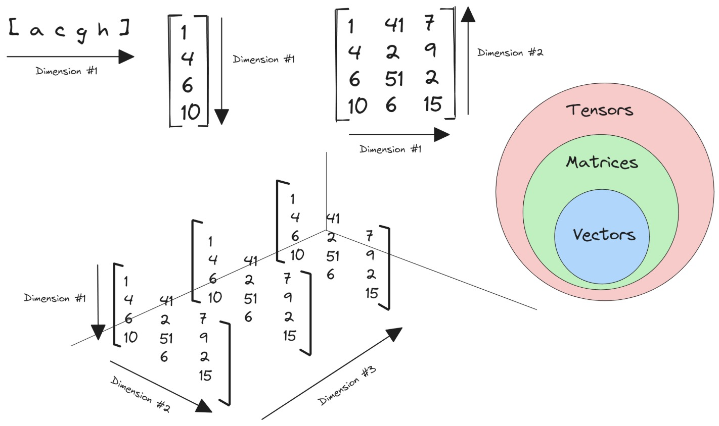
The Hierarchy: Scalar to N-D Tensor

NumPy provides the perfect bridge between mathematical concepts and computational reality with its ndarray (n-dimensional array).

Scalar (Rank 0)

import numpy as np

x = np.array(42)
print(x)
print(f'A scalar is of rank {x.ndim}')
# Output:
# 42
# A scalar is of rank 0

Vector (Rank 1)

x = np.array([1, 1, 2, 3, 5, 8])
print(x)
print(f'A vector is of rank {x.ndim}')
# Output:
# [1 1 2 3 5 8]
# A vector is of rank 1

Matrix (Rank 2)

x = np.array([[1, 4, 7],
              [2, 5, 8],
              [3, 6, 9]])
print(x)
print(f'A matrix is of rank {x.ndim}')
# Output:
# [[1 4 7]
#  [2 5 8]
#  [3 6 9]]
# A matrix is of rank 2

3D Tensor (Rank 3)

x = np.array([[[1, 4, 7],
               [2, 5, 8],
               [3, 6, 9]],
              
              [[10, 40, 70],
               [20, 50, 80],
               [30, 60, 90]],
              
              [[100, 400, 700],
               [200, 500, 800],
               [300, 600, 900]]])

print(x)
print(f'This tensor is of rank {x.ndim}')
# Output: This tensor is of rank 3

Important Distinction: Terminology

In practice, when we say “tensor” in ML, we typically mean rank-3 or higher to avoid confusion. Calling the scalar 42 a “tensor” is technically correct but not helpful.

Mathematically speaking, tensors are more than simply a data container. Aside from holding numeric data, tensors also include descriptions of the valid linear transformations between tensors (like cross product and dot product). From a computer science perspective, tensors can be thought of as objects in an object-oriented sense, not just data structures.

---

Tensors in PyTorch — The ML Practitioner’s Toolkit

PyTorch tensors are where theory meets practice in modern deep learning. They’re similar to NumPy arrays but with superpowers.

What Makes PyTorch Tensors Special?

From PyTorch’s documentation:

“Tensors are a specialized data structure that are very similar to arrays and matrices. In PyTorch, we use tensors to encode the inputs and outputs of a model, as well as the model’s parameters.”

PyTorch Tensor = NumPy Array + GPU Acceleration + Automatic Differentiation

Key differences from NumPy:

• Tensors can run on GPUs or other hardware accelerators
• Tensors and NumPy arrays can often share the same underlying memory
• Tensors are optimized for automatic differentiation (crucial for backpropagation)

Creating Tensors in PyTorch

1. Directly from Python Data

import torch
import numpy as np

# Directly from lists
data = [[1, 2], [3, 4]]
x_data = torch.tensor(data)
print(x_data)
# Output:
# tensor([[1, 2],
#         [3, 4]])

2. From NumPy Arrays

np_array = np.array(data)
x_np = torch.from_numpy(np_array)

# Tensors and NumPy arrays can share memory!
# Changes to one can affect the other (when on CPU)

3. From Another Tensor

x_ones = torch.ones_like(x_data)  # Retains shape, changes values
print(f"Ones Tensor:\n {x_ones}\n")

x_rand = torch.rand_like(x_data, dtype=torch.float)  # Override datatype
print(f"Random Tensor:\n {x_rand}\n")

4. With Specified Shapes

shape = (2, 3)  # 2 rows, 3 columns
rand_tensor = torch.rand(shape)
ones_tensor = torch.ones(shape)
zeros_tensor = torch.zeros(shape)

print(f"Random Tensor:\n {rand_tensor}\n")
print(f"Ones Tensor:\n {ones_tensor}\n")
print(f"Zeros Tensor:\n {zeros_tensor}")

# Output:
# Random Tensor:
#  tensor([[0.4122, 0.1048, 0.6723],
#          [0.0083, 0.1560, 0.6437]])
# 
# Ones Tensor:
#  tensor([[1., 1., 1.],
#          [1., 1., 1.]])
# 
# Zeros Tensor:
#  tensor([[0., 0., 0.],
#          [0., 0., 0.]])

Tensor Attributes: Shape, Datatype, Device

Every tensor has three crucial attributes:

tensor = torch.rand(3, 4)

print(f"Shape: {tensor.shape}")           # torch.Size([3, 4])
print(f"Datatype: {tensor.dtype}")        # torch.float32
print(f"Device: {tensor.device}")         # cuda, mps or cpu

These attributes tell you:

• Shape: The dimensions of the tensor
• Datatype: The data type of elements (float32, int64, etc.)
• Device: Where the tensor is stored (GPU or CPU)

Moving Tensors to GPU/Accelerator

One of PyTorch’s killer features is seamless CPU-GPU operations:

# Check for accelerator availability and move tensor
if torch.accelerator.is_available():
    tensor = tensor.to(torch.accelerator.current_accelerator())
    print(f"Device: {tensor.device}")  # cuda:0 or mps:0

# Or specifically for CUDA
if torch.cuda.is_available():
    tensor = tensor.to('cuda')

Copying large tensors across devices is expensive in terms of time and memory!

Essential Tensor Operations

PyTorch offers over 1200 tensor operations, including arithmetic, linear algebra, matrix manipulation, sampling, and more.

Indexing and Slicing (NumPy-style)

tensor = torch.ones(4, 4)

print(f"First row: {tensor[0]}")        # First row
print(f"First column: {tensor[:, 0]}")  # First column
print(f"Last column: {tensor[..., -1]}")  # Last column

# In-place modification
tensor[:, 1] = 0
print(tensor)
# Output:
# tensor([[1., 0., 1., 1.],
#         [1., 0., 1., 1.],
#         [1., 0., 1., 1.],
#         [1., 0., 1., 1.]])

Joining Tensors

# Concatenate along dimension 1 (columns)
t1 = torch.cat([tensor, tensor, tensor], dim=1)
print(t1)
# Output: 4 rows, 12 columns (3x the original width)

# Stack creates a new dimension
t2 = torch.stack([tensor, tensor, tensor], dim=0)
# Output: [3, 4, 4] - stacks along new first dimension

Arithmetic Operations

# Matrix multiplication
y1 = tensor @ tensor.T
y2 = tensor.matmul(tensor.T)

y3 = torch.rand_like(y1)
torch.matmul(tensor, tensor.T, out=y3)  # In-place result

# Element-wise product
z1 = tensor * tensor
z2 = tensor.mul(tensor)

z3 = torch.rand_like(tensor)
torch.mul(tensor, tensor, out=z3)  # In-place result

Single-element Tensors

# Aggregation to scalar
agg = tensor.sum()
agg_item = agg.item()  # Convert to Python number
print(agg_item, type(agg_item))  # 12.0 <class 'float'>

In-place Operations

# Operations with _ suffix modify tensors in-place
tensor.add_(5)  # Adds 5 to every element
tensor.mul_(2)  # Multiplies every element by 2

# Warning: In-place ops save memory but can cause issues
# with automatic differentiation!

Tensor Shapes in Deep Learning

Understanding tensor shapes is crucial for debugging neural networks:

Data Type	Tensor Shape	Description
Image (RGB)	[3, 224, 224]	3 channels, 224×224 pixels
Batch of Images	[32, 3, 224, 224]	32 images in batch
Text Sequence	[batch, seq_len]	Token IDs
Embeddings	[batch, seq_len, embed_dim]	Word vectors
Video	[batch, frames, channels, H, W]	Video clips

Common Tensor Transformations

Reshaping

x = torch.randn(8, 16)
y = x.view(4, 32)      # Must have same number of elements
                       # Must be contiguous in memory

z = x.reshape(2, 4, 16)  # More flexible, may copy data
                         # Works even if not contiguous

Permuting Dimensions

x = torch.randn(32, 3, 224, 224)  # [N, C, H, W]
x_perm = x.permute(0, 2, 3, 1)    # [N, H, W, C]
# Useful for converting between different frameworks

Squeezing and Unsqueezing

x = torch.randn(1, 28, 28)
y = x.squeeze(0)      # Remove dimension 0: [28, 28]
z = y.unsqueeze(0)    # Add dimension 0: [1, 28, 28]

# Common use: adding batch dimension
batch_x = x.unsqueeze(0)  # [1, 28, 28] -> [1, 1, 28, 28]

Broadcasting

# PyTorch automatically broadcasts tensors with compatible shapes
x = torch.randn(3, 4)
y = torch.randn(4)     # Can broadcast to [3, 4]
z = x + y              # y is broadcast to each row

# Broadcast rules:
# - Dimensions are aligned from right to left
# - Dimensions of size 1 can be broadcast to any size
# - Missing dimensions are added on the left

---

The ML Pipeline — Tensors in Action

Let’s see how tensors flow through a typical deep learning workflow:

Complete Example: Image Classification

import torch
import torch.nn as nn
import torch.nn.functional as F

# 1. Data as tensors
# Batch of 32 RGB images, 224x224 pixels
images = torch.randn(32, 3, 224, 224)  
labels = torch.randint(0, 1000, (32,))  # 32 class labels (ImageNet)

# 2. Model with tensor parameters
class SimpleConvNet(nn.Module):
    def __init__(self):
        super().__init__()
        self.conv1 = nn.Conv2d(3, 64, kernel_size=3, padding=1)
        self.conv2 = nn.Conv2d(64, 128, kernel_size=3, padding=1)
        self.pool = nn.MaxPool2d(2, 2)
        self.fc1 = nn.Linear(128 * 56 * 56, 512)
        self.fc2 = nn.Linear(512, 1000)
    
    def forward(self, x):
        # x: [32, 3, 224, 224]
        x = self.pool(F.relu(self.conv1(x)))  # [32, 64, 112, 112]
        x = self.pool(F.relu(self.conv2(x)))  # [32, 128, 56, 56]
        x = x.view(x.size(0), -1)             # [32, 128*56*56] flatten
        x = F.relu(self.fc1(x))                # [32, 512]
        x = self.fc2(x)                        # [32, 1000]
        return x

model = SimpleConvNet()

# 3. Forward pass: tensor operations
outputs = model(images)  # Shape: [32, 1000]
print(f"Output shape: {outputs.shape}")

# 4. Loss computation: tensor to scalar
criterion = nn.CrossEntropyLoss()
loss = criterion(outputs, labels)

print(f"Loss: {loss.item()}")  # Convert tensor to Python float

# 5. Backpropagation (automatic differentiation)
loss.backward()  # Computes gradients for all parameters

# 6. Access gradients (also tensors!)
for name, param in model.named_parameters():
    if param.grad is not None:
        print(f"{name}: {param.grad.shape}")

Common Tensor Operations in Deep Learning

Normalization

# Batch normalization expects [N, C, H, W]
x = torch.randn(32, 3, 224, 224)

# Normalize per channel
mean = x.mean(dim=[0, 2, 3], keepdim=True)  # [1, 3, 1, 1]
std = x.std(dim=[0, 2, 3], keepdim=True)
x_norm = (x - mean) / (std + 1e-5)

Attention Mechanism

# Simplified attention computation
batch, seq_len, d_model = 32, 128, 512

Q = torch.randn(batch, seq_len, d_model)  # Query
K = torch.randn(batch, seq_len, d_model)  # Key
V = torch.randn(batch, seq_len, d_model)  # Value

# Scaled dot-product attention
scores = torch.matmul(Q, K.transpose(-2, -1))  # [32, 128, 128]
scores = scores / (d_model ** 0.5)
attn_weights = F.softmax(scores, dim=-1)       # [32, 128, 128]
output = torch.matmul(attn_weights, V)         # [32, 128, 512]

Data Augmentation

# Example: Random horizontal flip
def random_flip(images):
    # images: [N, C, H, W]
    mask = torch.rand(images.size(0)) > 0.5
    images[mask] = torch.flip(images[mask], dims=[3])  # Flip width
    return images

augmented = random_flip(torch.randn(16, 3, 224, 224))

---

Part 5: Bridge to NumPy and Back

One of PyTorch’s strengths is easy interoperability with NumPy:

Converting Between PyTorch and NumPy

# NumPy to PyTorch
np_array = np.array([[1, 2], [3, 4]])
torch_tensor = torch.from_numpy(np_array)

# PyTorch to NumPy (CPU only)
torch_tensor = torch.tensor([[1, 2], [3, 4]])
np_array = torch_tensor.numpy()

# Important: They share memory!
np_array[0, 0] = 999
print(torch_tensor)  # Also changed!

GPU Tensors

# For GPU tensors, must move to CPU first
if torch.cuda.is_available():
    gpu_tensor = torch.randn(3, 3).cuda()
    np_array = gpu_tensor.cpu().numpy()

With Gradients

# Tensors with gradients need .detach()
x = torch.tensor([1., 2., 3.], requires_grad=True)
# np_array = x.numpy()  # Error!
np_array = x.detach().numpy()  # OK

---

Common Pitfalls and Best Practices

Shape Mismatches

# Common error
x = torch.randn(32, 3, 224, 224)
y = torch.randn(32, 1000)
# z = x + y  # Error! Shapes don't match

# Solution: Check shapes
print(f"x: {x.shape}, y: {y.shape}")

Memory Management

# Bad: Creates many intermediate tensors
result = tensor.cpu().numpy().tolist()

# Better: Minimize copies
result = tensor.tolist()  # Direct conversion

In-place Operations and Autograd

x = torch.tensor([1., 2., 3.], requires_grad=True)
# x += 1  # Can break autograd!
x = x + 1  # Safe

Device Mismatches

# Error: Tensors on different devices
cpu_tensor = torch.randn(3, 3)
if torch.cuda.is_available():
    gpu_tensor = torch.randn(3, 3).cuda()
    # result = cpu_tensor + gpu_tensor  # Error!
    result = cpu_tensor.cuda() + gpu_tensor  # OK

---

Practice Exercises

Exercise 1: Working with Real Images

Let’s see tensors in action with real image data. This example shows how to load an image, manipulate it as a tensor, and save the result.

import torch
from PIL import Image
import torchvision.transforms as transforms
import matplotlib.pyplot as plt

# 1. Load an image and convert it to a tensor
image_path = "test.jpg"
img = Image.open(image_path)

# Convert PIL Image to tensor [C, H, W] with values in [0, 1]
to_tensor = transforms.ToTensor()
img_tensor = to_tensor(img)

print(f"Image tensor shape: {img_tensor.shape}")  # e.g., torch.Size([3, 512, 512])
print(f"Data type: {img_tensor.dtype}")           # torch.float32
print(f"Value range: [{img_tensor.min():.3f}, {img_tensor.max():.3f}]")

# 2. Manipulate the tensor - let's apply some transformations

# Example A: Increase brightness by 30%
brightened = torch.clamp(img_tensor * 1.3, 0, 1)

# Example B: Convert to grayscale (weighted average of RGB channels)
# Standard formula: 0.299*R + 0.587*G + 0.114*B
weights = torch.tensor([0.299, 0.587, 0.114]).view(3, 1, 1)
grayscale = (img_tensor * weights).sum(dim=0, keepdim=True)
# Broadcast back to 3 channels for saving as RGB
grayscale_rgb = grayscale.repeat(3, 1, 1)

# Example C: Apply a color filter (boost red channel, reduce blue)
color_adjusted = img_tensor.clone()
color_adjusted[0] = torch.clamp(img_tensor[0] * 1.5, 0, 1)  # Red channel
color_adjusted[2] = torch.clamp(img_tensor[2] * 0.5, 0, 1)  # Blue channel

# Example D: Flip image horizontally (flip along width dimension)
flipped = torch.flip(img_tensor, dims=[2])

# Example E: Add some noise
noise = torch.randn_like(img_tensor) * 0.05
noisy = torch.clamp(img_tensor + noise, 0, 1)

# 3. Convert tensors back to PIL Images and save
to_pil = transforms.ToPILImage()

brightened_img = to_pil(brightened)
brightened_img.save("test_brightened.jpg")

grayscale_img = to_pil(grayscale_rgb)
grayscale_img.save("test_grayscale.jpg")

color_adjusted_img = to_pil(color_adjusted)
color_adjusted_img.save("test_color_adjusted.jpg")

flipped_img = to_pil(flipped)
flipped_img.save("test_flipped.jpg")

noisy_img = to_pil(noisy)
noisy_img.save("test_noisy.jpg")

print("\n✓ All manipulated images saved!")

# 4. Visualize the transformations (optional)
fig, axes = plt.subplots(2, 3, figsize=(15, 10))
axes = axes.flatten()

images_to_show = [
    (img_tensor, "Original"),
    (brightened, "Brightened (+30%)"),
    (grayscale_rgb, "Grayscale"),
    (color_adjusted, "Color Adjusted"),
    (flipped, "Flipped"),
    (noisy, "Noisy")
]

for ax, (tensor, title) in zip(axes, images_to_show):
    # Convert tensor [C, H, W] to [H, W, C] for matplotlib
    img_array = tensor.permute(1, 2, 0).numpy()
    ax.imshow(img_array)
    ax.set_title(title)
    ax.axis('off')

plt.tight_layout()
plt.savefig("tensor_transformations.png", dpi=150, bbox_inches='tight')
print("✓ Visualization saved as tensor_transformations.png")

Key Concepts Demonstrated:

• Loading: PIL Image → Tensor with shape [C, H, W]
• Tensor operations: Broadcasting, channel manipulation, mathematical operations
• Clamping: Keeping values in valid range [0, 1]
• Shape manipulation: .repeat(), .permute(), .flip()
• Saving: Tensor → PIL Image → File

Exercise 2: Batch Processing Multiple Images

import torch
from PIL import Image
import torchvision.transforms as transforms
from pathlib import Path

# Batch process multiple images
image_files = ["test.jpg", "image2.jpg", "image3.jpg"]

# Create a batch of tensors
batch_tensors = []
transform = transforms.Compose([
    transforms.Resize((224, 224)),  # Standardize size
    transforms.ToTensor()
])

for img_file in image_files:
    if Path(img_file).exists():
        img = Image.open(img_file)
        tensor = transform(img)
        batch_tensors.append(tensor)

# Stack into a single batch tensor [N, C, H, W]
if batch_tensors:
    batch = torch.stack(batch_tensors)
    print(f"Batch shape: {batch.shape}")  # e.g., torch.Size([3, 3, 224, 224])
    
    # Apply transformation to entire batch
    # Example: Normalize using ImageNet statistics
    mean = torch.tensor([0.485, 0.456, 0.406]).view(1, 3, 1, 1)
    std = torch.tensor([0.229, 0.224, 0.225]).view(1, 3, 1, 1)
    normalized_batch = (batch - mean) / std
    
    print(f"Normalized batch statistics:")
    print(f"  Mean per channel: {normalized_batch.mean(dim=[0, 2, 3])}")
    print(f"  Std per channel: {normalized_batch.std(dim=[0, 2, 3])}")

Exercise 3: Understanding Tensor Shapes with Images

import torch

# Create a batch of 16 random "images" (3 channels, 64x64)
images = torch.randn(16, 3, 64, 64)

print("Original shape:", images.shape)  # torch.Size([16, 3, 64, 64])

# 1. Calculate the mean per channel across the batch
channel_means = images.mean(dim=[0, 2, 3])
print(f"Channel means: {channel_means}")  # Shape: [3]

# 2. Normalize each channel
for c in range(3):
    images[:, c] = (images[:, c] - channel_means[c])

# 3. Reshape to a sequence (flatten spatial dimensions)
sequences = images.view(16, 3, -1)  # [16, 3, 4096]
print(f"Sequence shape: {sequences.shape}")

# 4. Calculate attention-like scores
Q = K = sequences
scores = torch.bmm(Q, K.transpose(1, 2))  # [16, 3, 3]
print(f"Attention scores shape: {scores.shape}")

# 5. Common shape transformations
print("\n--- Shape Transformations ---")
print(f"Original: {images.shape}")
print(f"Flattened: {images.flatten().shape}")  # All dims → 1D
print(f"Permuted (NHWC): {images.permute(0, 2, 3, 1).shape}")  # [N,C,H,W] → [N,H,W,C]
print(f"Squeezed: {images[:1].squeeze().shape}")  # Remove batch dim if size 1
print(f"Unsqueezed: {images.unsqueeze(0).shape}")  # Add new dim at front

The Big Picture:

Every deep learning model is just tensors flowing through differentiable operations:

Image File → Tensor → Neural Network → Output Tensor → Prediction
   (disk)     [N,C,H,W]   (matrix ops)    [N, classes]    (argmax)

Master tensors, master deep learning.