Yes, You Should Understand Backprop: A Step-by-Step Walkthrough
Backpropagation—originating in Linnainmaa’s 1970 reverse-mode AD thesis and popularized for neural nets by Rumelhart et al. in 1986—is the workhorse that makes deep learning feasible (en.wikipedia.org, de.wikipedia.org). It efficiently computes gradients via a reverse traversal of a computation graph, applying the chain rule at each node (colah.github.io, cs231n.stanford.edu).
Understanding its mechanics by hand helps you debug and improve models when “autograd” breaks down—Karpathy warns that leaky abstractions hide vanishing/exploding gradients and dying ReLUs unless you look under the hood (karpathy.medium.com, cs231n.stanford.edu).
We’ll cover its history, intuition, vectorized formulas, a worked numeric example, common pitfalls, and modern remedies—with pointers to every key paper and lecture.
Introduction
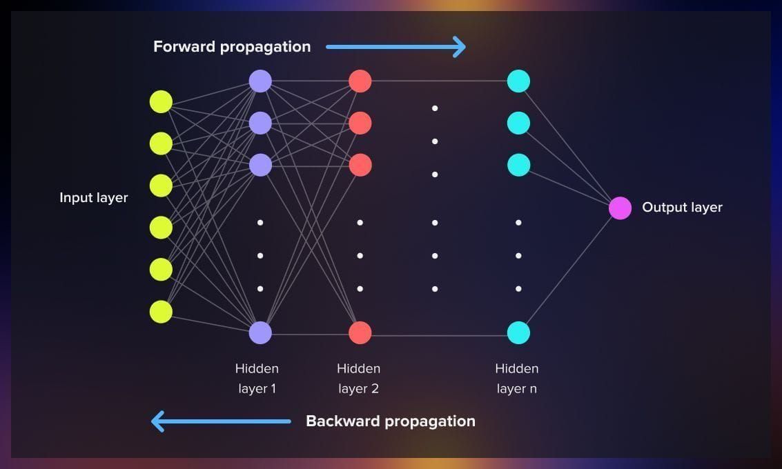
Backpropagation is the algorithm that computes the gradient of a scalar loss $L$ with respect to all network parameters by recursively applying the chain rule from outputs back to inputs (colah.github.io, cs231n.stanford.edu).
In code, frameworks like TensorFlow or PyTorch automate backward passes, but treating it as a black box can obscure subtle failure modes—debugging requires tracing error signals through each operation (karpathy.medium.com).
A Brief History of Backpropagation
1. 1970: Reverse-Mode Automatic Differentiation
Seppo Linnainmaa’s 1970 M.Sc. thesis introduced “reverse-mode” AD: representing a composite function as a graph and computing its derivative by a backward sweep of local chain-rule applications (en.wikipedia.org, idsia.ch).
2. 1974–1982: From AD to Neural Nets
Paul Werbos recognized that reverse-mode AD could train multi-layer perceptrons, presenting this idea in his 1974 Harvard PhD and later publications (news.ycombinator.com).
3. 1986: Rumelhart, Hinton & Williams
David Rumelhart, Geoff Hinton & Ronald Williams formalized backpropagation for neural networks in their landmark Nature paper, showing multi-layer nets could learn internal representations (en.wikipedia.org).
4. 2000s: The Deep Learning Boom
GPUs, large datasets, and architectural innovations (CNNs, RNNs) made deep nets practical. Backprop—once limited to shallow networks—now trains architectures with hundreds of layers (colah.github.io, jmlr.org).
Why You Must Understand Backprop by Hand
Even though autograd handles derivatives, Karpathy stresses that treating backprop as “magic” leads to leaky abstractions—you’ll miss why your model stalls, diverges, or suffers dead neurons (karpathy.medium.com).
Engineers who can manually step through a backward sweep catch vanishing/exploding gradients and activation pitfalls early, saving days of debugging.
How Backpropagation Actually Works
A. Computation Graphs & the Chain Rule
Every operation in a network is a node in a directed acyclic graph. Given $y = f(x)$ and a loss $L$, the backward step computes
\[\frac{\partial L}{\partial x} = \frac{\partial L}{\partial y}\;\frac{\partial y}{\partial x},\]re-using $\partial L/\partial y$ as the “upstream” signal at each edge (colah.github.io, cs231n.stanford.edu).
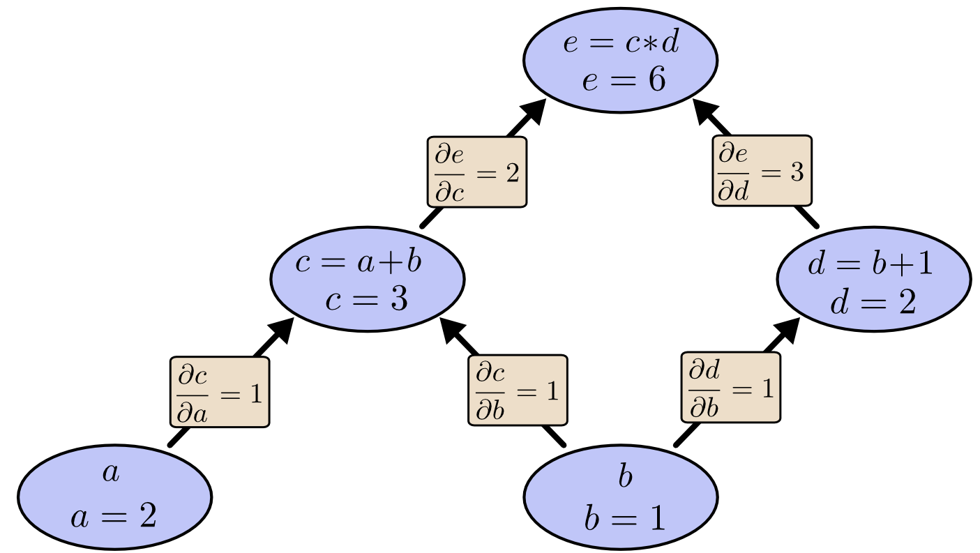 simple chain-rule graph, source: Calculus on Computational Graphs: Backpropagation
B. Vectorized Layer-Wise Updates
For a fully-connected layer $l$ with inputs $a^{l-1}$, pre-activations $z^l=W^l a^{l-1}+b^l$, activations $a^l=f(z^l)$, and loss gradient $\delta^l = \partial L/\partial z^l$, the updates are:
\[\nabla_{W^l}L = \delta^l\, (a^{l-1})^T,\quad \nabla_{b^l}L = \sum_i \delta^l_i,\quad \delta^{l-1} = (W^l)^T\,\delta^l \;\circ\; f'(z^{l-1})\]where $\circ$ is element-wise multiplication (cs231n.stanford.edu, cs231n.github.io).
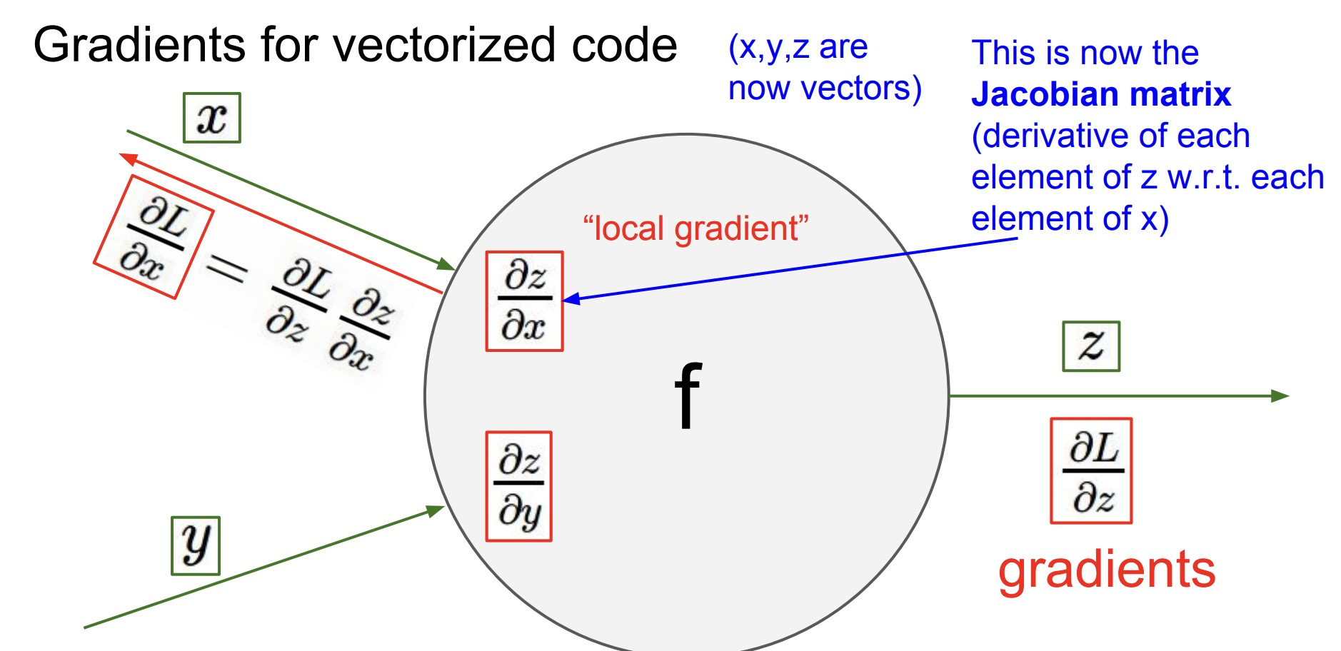 vectorized backprop, source: [CS231N slide 53][https://cs231n.stanford.edu/slides/2017/cs231n_2017_lecture4.pdf]
C. Worked Numerical Example
Matt Mazur’s two-layer network example crunches actual numbers—forward activations to (0.01, 0.99) and backward gradients to concrete $\Delta W$, $\Delta b$ updates. Stepping through it cements intuition (colah.github.io, web.stanford.edu).
Pitfalls & Practical Tips
1. Vanishing & Exploding Gradients
Sigmoid/tanh saturation ($f’(z)\to0$) shrinks gradients exponentially in depth; poor initialization can blow them up. Use Xavier/He initialization and, for RNNs, gradient clipping (karpathy.medium.com, cs231n.stanford.edu).
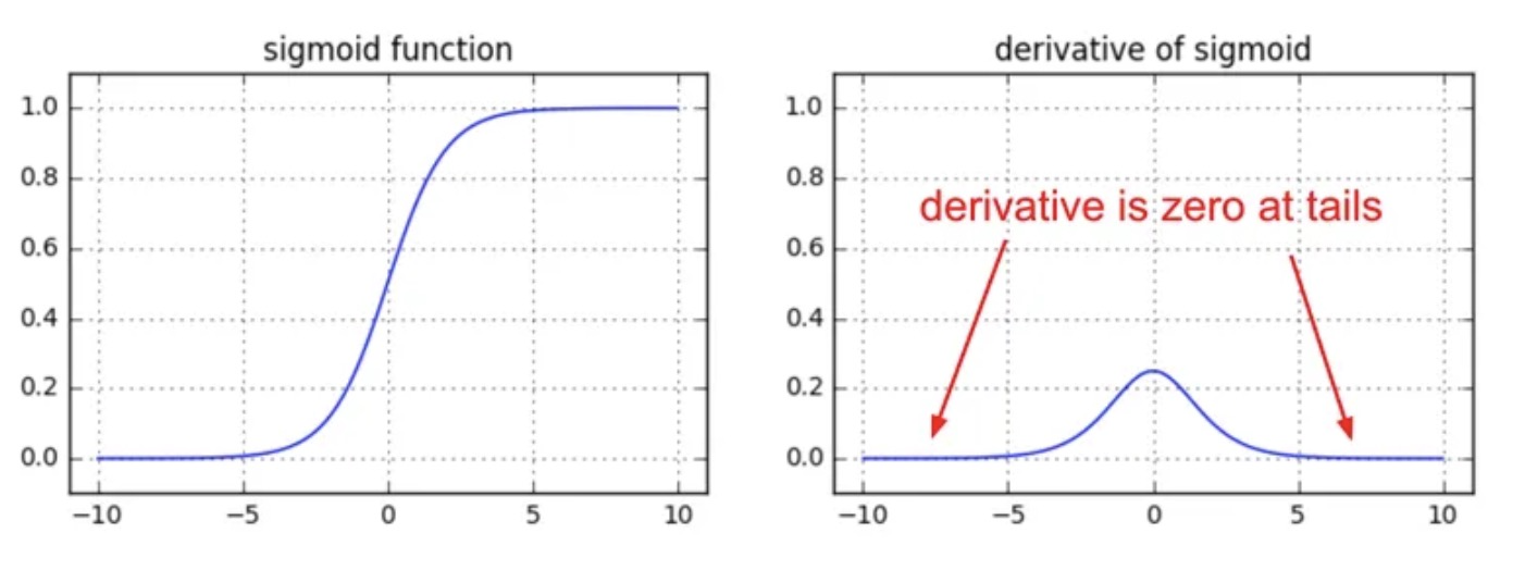 Sigmoid derivative vanishing plot, source: karpathy.medium.com
2. Dying ReLUs
ReLUs zero-out for negative inputs; if a neuron’s gradient path stays negative, it “dies.” Karpathy calls this “brain damage.” Leaky-ReLU, PReLU or ELU keep a small slope for $z<0$ (karpathy.medium.com, substack.com).
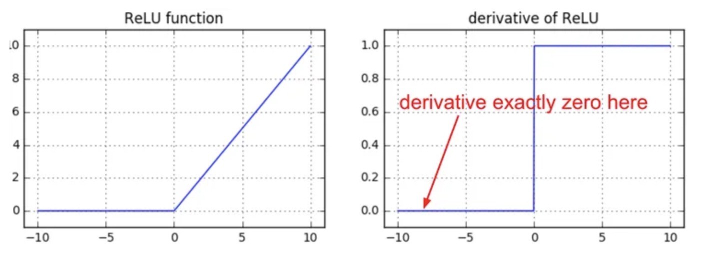 ReLU zero-slope region, source: karpathy.medium.com
3. Modern Remedies
Batch normalization, residual/skip connections (ResNets), and newer activations (SELU) preserve signal flow in very deep nets (karpathy.medium.com, jmlr.org).
Conclusion & Further Reading
A hands-on grasp of backpropagation is essential for debugging, architecture design, and research innovation. For deeper dives, see:
- Collobert & Weston, “Natural Language Processing (Almost) from Scratch” (JMLR 2011) (jmlr.org)
- CS231n “Derivatives, Backpropagation, and Vectorization” handout (cs231n.stanford.edu)
- Nielsen, Neural Networks and Deep Learning, Ch. 2
- Olah, “Calculus on Computational Graphs: Backpropagation” (colah.github.io)
- Inna Logunova, Backpropagation in Neural Networks
Need Help with Your AI Project?
Whether you’re building a new AI solution or scaling an existing one, I can help. Book a free consultation to discuss your project.