Fine-tuning a large language model depends on optimizing several key hyperparameters to unlock its full potential. In this discussion, we focus on the three most important hyperparameters – batch size, learning rate, and epochs. By carefully adjusting these hyperparameters to match your specific use case, you can achieve an ideal balance between training speed, memory consumption, and overall model accuracy.
Batch Size
The batch size is how many training samples you process in a single forward-backward pass cycle before updating the model’s parameters. For example:
- Batch Size = 1: The model sees only one row of your training data at a time and immediately updates the model’s weights based on that single training data loss.
- Batch Size = 2 (or more): The model processes multiple examples at once, and averages the losses from all of them before performing a single parameter update.
GPUs excel at parallel processing, so feeding several rows simultaneously allows for an efficient forward pass across these rows.
Understanding batch size is crucial for effectively fine-tuning your model and achieving your desired outcomes. It’s important to recognize the difference between performing a backward pass immediately after processing a single sample versus aggregating the forward passes from multiple samples and then computing a single backward pass on their combined loss.
Let’s examine two scenarios to illustrate this distinction.
Case 1: Batch Size = 1
When using a batch size of 1, the model processes and updates its weights based on one training sample at a time. Imagine the model’s weights are represented as a point on a multi-dimensional loss surface:
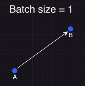
First Training Sample:
The model starts at point A (its initial set of weights). It processes the first row of training data through a forward pass, predicting the next tokens. The predicted tokens are then compared with the actual tokens, and the loss is calculated. This loss is backpropagated through the network, updating the model’s weights and moving them from point A to point B.
Second Training Sample:
The model now begins at point B (the updated weights from the first sample). It processes the second row of training data, computes the loss based on its predictions versus the actual tokens, and backpropagates this loss. The weights are updated again, moving the model from point B to point C.
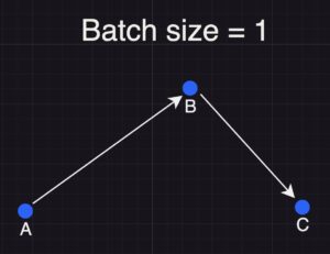
In essence, with a batch size of 1, each training sample independently influences the model’s weight update, resulting in a sequential trajectory across the loss surface.
Case 2: Batch Size = 2
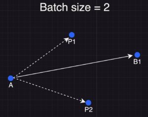
When using a batch size of 2, the model processes two training samples simultaneously rather than one after the other. Imagine the model’s weights start at point A. Now, instead of handling one row at a time, the model performs a forward pass on both rows in parallel. Each sample independently generates its predictions (P1 and P2), and the losses from both samples are calculated. These individual losses are then summed and then averaged to form a single aggregate loss.
This combined loss represents the net effect of both samples together. Instead of updating the weights first from A to B (based on the first row) and then from B to C (based on the second row) as in the sequential approach, the model takes one update step based on the aggregated loss (P1+P2). This single step moves the model’s weights from point A directly to a new point (let’s call it B1) on the loss surface. Note that point B1 is not equivalent to the sequential update you’d get by processing the samples individually; rather, it reflects the average direction suggested by both samples.
To reiterate, when you use a batch size of one, the model’s weights are updated individually for each row of training data. In this approach, the model explores the loss surface one sample at a time—each update is highly specific to the information contained in that single row.
In contrast, when the batch size is increased, the losses from multiple rows are combined—typically by summing and averaging—to compute a single aggregate loss. The model then takes one update step based on this combined loss, effectively averaging the update directions from the individual samples. This averaging reduces the noise inherent in any one sample, leading to more stable and consistent updates across the training process.
However, there is a trade-off. With larger batch sizes, the update reflects an averaged signal rather than the unique details of each row. For instance, if one sample emphasizes the “apple harvest season” and another focuses on “pineapples,” the resulting update will be a blend of both signals instead of capturing each detail separately. Consequently, if you need very precise, row-specific updates—say, to memorize unique or nuanced information—a batch size of one might be preferable. Conversely, when training on a very large dataset, combining multiple samples per update can help improve training speed and stability by smoothing out the noise.
To sum it all up, the benefits and drawbacks of using a smaller batch size are as follows:
Benefits of a Smaller Batch Size:
- More Granular Learning: Since the model updates its weights after processing each individual sample, the learning process is very precise, allowing the model to fit the data in a highly specific, stepwise manner.
- Reduced Memory Usage: Smaller batch sizes require less VRAM, which means you need less GPU memory since you’re processing fewer samples at a time.
Downsides of a Smaller Batch Size:
- Slower Training: Because updates occur more frequently (i.e., after every single row), the overall training process tends to be slower.
- Higher Overfitting Risk: With very specific updates for each row, the model may become too finely tuned to the training data, potentially leading to overfitting.
On the other hand, increasing the batch size comes at a cost in memory usage. You can estimate the memory requirement with the following formula:
Total memory = model parameters + (batch size × memory per sample)
This formula shows that the total GPU memory needed is the sum of the memory required to load the model and the memory needed for a single batch in its tokenized format.
Learning Rate
When fine-tuning an LLM using supervised fine-tuning (SFT), a common starting point for the learning rate is around 1e-4. This value generally offers a good balance: it allows the model to adjust its weights significantly with each update without causing instability. Here’s some guidance on managing the learning rate during fine-tuning:
- Start at 1e-4:
This is a typical baseline for fine-tuning LLMs. If your training and validation loss curves are smooth, you might have some room to increase the learning rate slightly. Conversely, if you observe that the loss—especially the validation loss—is fluctuating wildly, it’s a sign that the learning rate may be too high, and you should consider lowering it. - Monitor Loss Behavior:
- If the training loss fluctuates excessively, reduce the learning rate (e.g., try lowering it to 1e-5) to stabilize the updates.
- If the loss is extremely smooth and convergence is slow, you can increase the learning rate slightly to speed up training.
- Learning Rate Schedules:
Implementing a learning rate schedule—such as starting with a warm-up phase followed by linear decay—can further enhance training stability. The warm-up phase helps the model begin training gently, while decay ensures the learning rate decreases as the model converges.
Number of Epochs
Finding the optimal number of epochs is a balancing act:
- Initial Runs:
Start your training runs with a constant (flat) learning rate. This allows you to establish a baseline without the added complexity of a changing learning rate. - Monitoring Validation Loss:
As you train over multiple epochs, keep a close eye on your validation loss. Typically, during early epochs the loss decreases steadily. However, after a certain point, you might notice the validation loss starting to increase—a clear indicator that the model is beginning to overfit. - Determining the “Sweet Spot”:
For example, if your evaluation loss starts to rise after two epochs, that’s a useful data point. You can note down that epoch number as a candidate for early stopping. - Refinement With Learning Rate Schedules:
Once you identify the approximate point where overfitting begins, try rerunning the training using a learning rate schedule—such as cosine annealing or linear decay. These methods gradually reduce the learning rate as training progresses, allowing the model to take increasingly smaller steps as it nears a local minimum. This fine-tuning can help you get closer to the optimal convergence point without overshooting.
Experimentation Is Key
The ideal number of epochs depends on your dataset, model architecture, and the specific task at hand. For short training runs where you can afford multiple experiments:
- Run Multiple Trials:
Experiment with a constant learning rate to first determine when your validation loss begins to climb. - Adjust and Rerun:
Once you have that baseline, adjust your learning rate schedule (for example, switching from constant to cosine or linear decay) to see if you can train for slightly longer while still avoiding overfitting. - Balance Overfitting and Underfitting:
Too few epochs might lead to underfitting, where the model hasn’t learned enough, while too many epochs can cause overfitting, where the model learns the noise in the training data.
Final Thoughts
Opt for a batch size that balances your memory constraints and training efficiency. While smaller batch sizes offer more granular updates and require less GPU memory, they can slow down training and may increase the risk of overfitting. Conversely, larger batch sizes, though more memory-intensive, can provide more stable updates by averaging over multiple samples. Experiment with different batch sizes to find the optimal balance for your specific use case.
Choosing an appropriate learning rate—and adjusting it dynamically during training—can help balance rapid initial learning with stable, gradual convergence, ultimately leading to better model generalization.
Choosing the number of training epochs isn’t just about stopping at the first sign of overfitting; it’s about understanding your model’s learning curve and making adjustments accordingly. By monitoring validation loss closely and experimenting with learning rate schedules, you can identify that sweet spot where the model has learned enough from the data while still maintaining its ability to generalize.
When fine-tuning an LLM, selecting the right pre-trained model is as important as optimizing your hyperparameters. Before you begin, evaluate potential models based on their pre-training domain, architecture, and scale to ensure they align with your specific task. A model that has already demonstrated strong performance in your domain can often serve as a better starting point, reducing both fine-tuning time and resource requirements.
This might sound obvious, but before you invest in fine-tuning, test a few different models in their raw, un-tuned state. For example, if your application is focused on vintage car restoration, try asking sample questions to raw versions of your LLMs candidates. You may find that the model performing best out of the box isn’t necessarily the strongest overall—it might simply have been trained on data that overlaps well with the knowledge you want to refine. Starting with the model that naturally performs best on your task can simplify the fine-tuning process and yield better results.
Throughout the fine-tuning process, it’s essential to keep a close eye on your training and validation losses. As discussed, validation loss is a key indicator of overfitting or underfitting, while fluctuations in training loss can provide early clues about the model’s convergence behavior. Tools like TensorBoard are invaluable for visualizing these metrics in real-time, allowing you to adjust your learning rate, batch size, and epoch count as needed. In a future article, I’ll show you how to set up and effectively use these visualization tools.
By balancing the selection of the right LLM with careful hyperparameter tuning and robust monitoring, you can optimize your model’s performance and ensure it generalizes well to your specific use case.