Data visualization is far more than a pretty picture. In high-dimensional spaces (like the 784-dimensional MNIST images), a simple numeric accuracy score doesn’t always reveal which classes might be easily confused by your model. By reducing and plotting your data (using methods such as t-SNE, UMAP, or PCA), you can see how the model clusters or separates each class.
A classic example from MNIST is that 1’s can look suspiciously like 7’s—especially if someone writes 7 with a minimal crossbar or a slightly slanted 1. Even if your model scores high overall accuracy, you might see in the embedding visualization that many 1’s and 7’s end up clustered together. That indicates the model is more likely to mix them up.
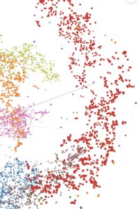
In the picture below notice how close some some orange dots (7) and some red dots (1) are
This phenomenon has been widely discussed in ML circles.
Key Benefits of Visualizing
-
Spotting Overlaps:
If two classes cluster together (like 1 and 7), your model is prone to confusion in that region of the input space. -
Debugging Mislabeled Data:
Sometimes you’ll see an “outlier” digit 9 among 4’s, which might actually be mislabeled. -
Model Interpretation:
A well-separated embedding often means your model is learning robust, distinct features. Overlapping clusters can signal where it struggles.
Example: MNIST Embeddings in TensorBoard
Below is a code snippet that generates an embedding for the MNIST test set, writes out a metadata file for the labels, and then uses TensorBoard’s Projector to visualize them. The snippet uses TF1-style code with disable_eager_execution to ensure the Projector reads the labels correctly.
import os
import numpy as np
import tensorflow as tf
import tensorflow_datasets as tfds
from tensorboard.plugins import projector

# Disable eager execution so we can use TF1-style summary writer.
tf.compat.v1.disable_eager_execution()

# Define log directory and metadata file
LOG_DIR = os.path.join(os.getcwd(), 'mnist-tensorboard', 'log-1')
os.makedirs(LOG_DIR, exist_ok=True)
metadata_path = os.path.join(LOG_DIR, 'metadata.tsv')

# Load MNIST test dataset with as_supervised=True (returns image, label pairs)
ds_test = tfds.load('mnist', split='test', as_supervised=True)

# Collect a fixed number of examples for visualization
images = []
labels = []
for image, label in tfds.as_numpy(ds_test.take(10000)):
    images.append(image.reshape(-1))  # flatten 28x28 image
    labels.append(label)
images = np.array(images)

# Create a TensorFlow variable for the embeddings
embedding_var = tf.Variable(images, name='embedding')

# Write out the metadata file (add header and 10,000 label lines -> 10001 total lines)
with open(metadata_path, 'w') as f:
    f.write("label\n")
    for label in labels:
        f.write(f"{label}\n")

# Save the checkpoint for the embedding variable
saver = tf.compat.v1.train.Saver([embedding_var])
with tf.compat.v1.Session() as sess:
    sess.run(tf.compat.v1.global_variables_initializer())
    saver.save(sess, os.path.join(LOG_DIR, "embedding.ckpt"))

    # Configure the projector
    config = projector.ProjectorConfig()
    embedding = config.embeddings.add()
    embedding.tensor_name = embedding_var.name
    # Use an absolute path for the metadata
    embedding.metadata_path = os.path.abspath(metadata_path)

    # Use a TF1 summary writer
    writer = tf.compat.v1.summary.FileWriter(LOG_DIR, sess.graph)
    projector.visualize_embeddings(writer, config)
    writer.close()

print("Setup complete. Launch TensorBoard with:")
print(f"tensorboard --logdir={LOG_DIR}")
Code Explanation
-
Data Loading:
We loadmnistfromtfds(TensorFlow Datasets) withsplit='test'. Theas_supervised=Trueflag yields(image, label)pairs. -
Preprocessing:
- Each
imageis reshaped from(28, 28)to a single 1D array of length 784. - We collect
labelsin a parallel list.
- Each
-
Creating the Embedding Variable:
embedding_var = tf.Variable(images, name='embedding')is the data we’ll visualize in the projector. -
Metadata File:
- We open
metadata.tsvand write a header line,"label". - Then we write each label on its own line. This ensures TensorBoard knows there’s a column called
labelfor coloring.
- We open
-
Saving the Checkpoint:
We usetf.compat.v1.train.Saverto save the variable’s values inembedding.ckpt. TensorBoard will read this checkpoint at runtime. -
Projector Config:
embedding.tensor_name = embedding_var.nametells the projector which variable to visualize.embedding.metadata_path = os.path.abspath(metadata_path)ensures the metadata file is found.
-
Summary Writer:
- We create a TF1-style summary writer (
FileWriter), passing insess.graph. projector.visualize_embeddings(writer, config)writes out aprojector_config.pbtxtthat TensorBoard uses.
- We create a TF1-style summary writer (
-
TensorBoard:
- Finally, we close the writer and print the command to run:
tensorboard --logdir=mnist-tensorboard/log-1
Wrap-Up
When you open TensorBoard’s “Projector” tab, you’ll see how the digits cluster in 2D/3D. Look for areas where 1’s and 7’s overlap—they can be visually similar. This overlap might indicate potential misclassifications, reminding you that data visualization can reveal subtle pitfalls that raw accuracy doesn’t always capture.
I hope you find this simple introduction helpful. As always, you can download the full source code [edit] I moved all the code on my GitHub repo
Happy embedding—and watch out for those tricky 1’s and 7’s!